 |
Tolerance accumulator
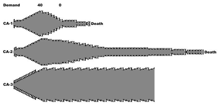
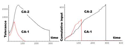
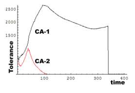
We explore the properties of the tolerance accumulator which was introduced in the previous experiment . The proliferon consists of a stem CA-0, CA-1 and CA-2. CA-2 gets resources from CA-1 and accumulates them. In the previous experiment demand oscillated. Here demand rises to a maximum = 40 and then declines to zero not to rise again.
delivery[2, 1, k, 2] ;
delivery[2, 2, k, 2] ;
If[ p[1,prev] > p[1,now], set rule[250]]; Min[++k,
40], else [set rule[600]]
Before the experiment started CA-0 planted two zygotes
which grew into mature isolated CA. When the experiment begins demand
starts rising. CA-1 and CA-2 switch between rules 600 and 250. as
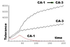
described before. CA-2 and CA-3 are accumulators.
 |
 |
 |
 |
CA-3 is an accumulator which does not depend on demand. It produces tolerance and accumulates it (middle curve). delivery[3, 3, 40, 2]. In addition it may accumulate tolerance delivered to it by CA-1 (upper curve). [3, 1, 40, 2]
 |
Mutual interaction
Compare this experiment with a two compartment model. Y1 contains resources and delivers them to Y2 which delivers them to the environment. Their relationship is described by two differential equations.
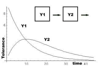 |
Y2 is a passive container which receives and delivers. The left arrow stands for a constant rate of delivery from Y1 to Y2. In the above experiment each compartment is a process (CA). The arrow indicates more than just a constant transfer rate of resources. It actually triggers Y2.
delivery:
[j, j-1, While[p[j-1] > set point], 2]
Argument[1]: Activated CA.
Argument[2]: Activating CA.
Argument[3]: Delivery condition.
Argument[4]: Delivery amount.
p[j]: daily production