 |
Rising demand-2
delivery[1, 1, k, 2]
{k, 20, 70}
If[ p[1,prev] > p[1,now], augment[1,
0, 0]]
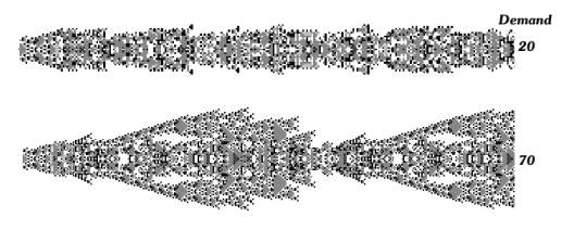
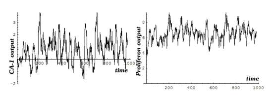
The image depicts two CA exposed respectively to demands
= 20 and 70.
 |
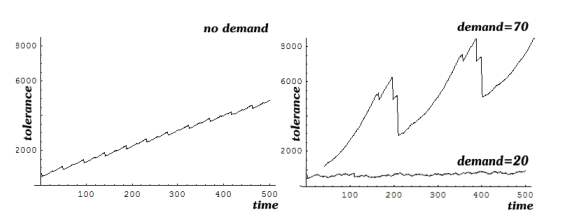
The left graph depicts tolerance accumulation of the
isolated stem process (CA-0). At low demand CA-1 accumulated less tolerance
than CA-0 (right graph). As demand rose, CA-1 accumulated more and more
tolerance and became vigorous.
 |
Despite its weak physique already at a demand of 20, CA-1 delivered twice as much as CA-0. The graph depicts CA-1 output as a multiple of CA-0 output. Health is expressed in relation with the isolated CA-0 whose health = 0.
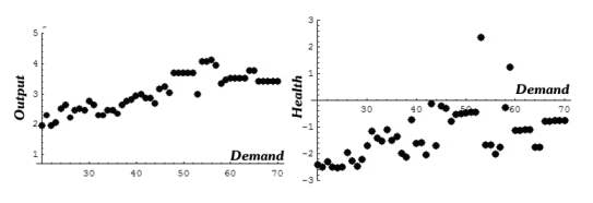 |
Even a small demand deteriorates CA-1
health, since CA-1 diverts some of its resources to the output, accumulates less tolerance, and its health is
low (fragile). As demand rises CA-1 adapts better and better.
Demand in an ongoing CA
If[ p[1,prev] > p[1,now], augment[1,
0, 0]; Min[++k, 70]]
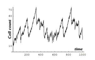
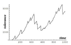
The next image depicts CA-1 cell count.
CA-1 starts as an isolated process. At time = 20 it enters a transient
phase during which it reacts to the rising demand. When
demand reaches 70 CA-1 settles at an attractor and starts oscillating.
 |
 |
 |
The experiment illustrates again that interaction with the environment, like demand, rescues the CA from isolation. It starts differentiating and when it attains its solution (attractor) it delivers as much as it can. It delivers and its tolerance declines. Then it pauses to regain its breath, delivers again and so on.
delivery:
[j, j-1, While[p[j-1] > set point], 2]
Argument[1]: Activated CA.
Argument[2]: Activating CA.
Argument[3]: Delivery condition.
Argument[4]: Delivery amount.
p[j]: daily production
Argument[1]: Augmented CA.
Argument[2]: Augmenting CA.
Argument[3]: Delivery condition.
p[j, now]: daily
production.
p[j, prev]: yesterdays
production.