Tolerance acceleration

The previous experiment computed the maximal tolerance accumulation rate of a two CA proliferon. Despite delivering some of its resources into the environment, CA-1 succeeded accumulating some tolerance. With aid of the delivery activation:  [1, 0, set point = p[1]-0.1,state[0,43]]  and change state: [state[1, i+1] = state[0. i], state[0, 43]]  it was possible to find the coordinates of a CA-1 with the fastest tolerance accumulation.  Its coordinates are {43,42}.

First let’s explain the functions involved in the computation:

augment state: [state[j, i+1] += state[j-1, i], state[0, k]];  {k,1,46}

First argument: CA-j state augmentation.
Second argument: CA-0 state which activates the augmentation.

delivery activation: [state[j , set point = p[j] - 0.1, state[0,43]]

First argument: CA-j which is activated.
Second argument: set point definition.
Third argument: CA-0 state which activates delivery.
p[j]:  daily CA-j production.

delivery: [j, j-1, While[p[j-1] > set point], 2]

First argument: CA-j receiving the delivery. 
Second argument: CA-j-1 delivering the product.
Third argument: Delivery condition.
Fourth argument: Delivery amount.
p[j]:  CA-j daily production.

change state: [state[j, i+1] = state[0. i], state[0, k]] {k, 1, 46}
First argument: state transfer from CA-0 to CA-j
Second argument: CA-0 state which activates the change.

In the present experiment CA-1 consists of a three CA proliferon: CA-0 controls CA-1 and CA-2. CA-1 delivers resources to CA-2, which does not deliver resources. CA-0 and CA-1 accumulate tolerance at a constant rate. We shall therefore focus on CA-3.  The function settings are:

delivery activation: [state[1, set point = p[1] - 0.1, state[0, 43]]; Only CA-1 delivers. CA-2 is not activated and does not deliver.
delivery: [2,1, While[p[1] > set point], 2] 
change state: [state[1, i+1] = state[0. i], state[0, 43]]; CA-1 maintains its structure.
change state: [state[3, i+1] = state[0. i], state[0, k]] {k, 1, 46}
augment state: [state[2, i+1] += state[1, i], state[0, k]]  {k,1,46}

These were the settings of the previous computation:

delivery activation: [state[1, set point = p[1] - 0.1, state[0, k]] {k,1,46}
delivery: [1,1, While[p[1] > set point]: 2]  {delivers into the environment}
change state: [state[1, i+1] = state[0. i], state[0, k]] {k, 1, 46}

The image depicts the CA-1 donor whose  structure dos not change. CA-2 initial structure (isolated) and its structure at the maximum of the tolerance surface.

Tolerance accumulation rates

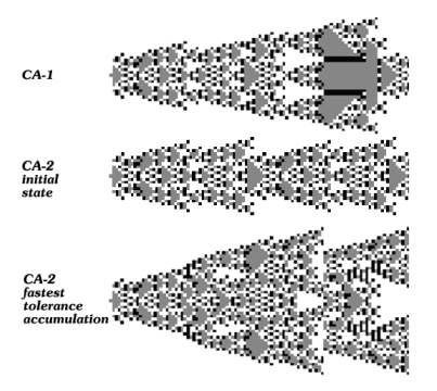
The surface depicts tolerance rates of 46 * 46 solutions. The central plain is occupied by isolated CA in which delivery was not activated and augment state was not effective. Even in their isolated state they accumulate tolerance at varying rates. Below this plain tolerance accumulation rate declines. (v. Tolerance accumulation. We may now ask what combination of CA states accumulates tolerance fastest? 

The graph below depicts accumulation rates maxima, many are higher than that of the previous experiment.

In the set of maximal tolerance rates, the overall mean daily tolerance gain above the isolated state (= 9.79) was 60.5 units (14.60 units in the previous experiment.

Tolerance acceleration

The surface depicts the average daily tolerance accumulation rate during steady state (homeorhesis. The overall tolerance of the present CA system  rises faster than that of the previous one.   The above function sets controlling the CA system generate two steady state configurations. Tolerance accumulation rates of both systems are constant. (They cruise in the tolerance space at two constant velocities). Actually the function set applied here accelerates the previous system to a new and healthier homeorhesis.