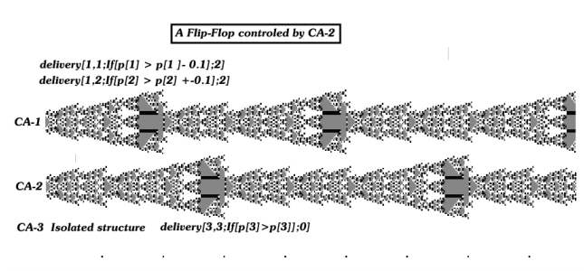
A non-linear flip-flop

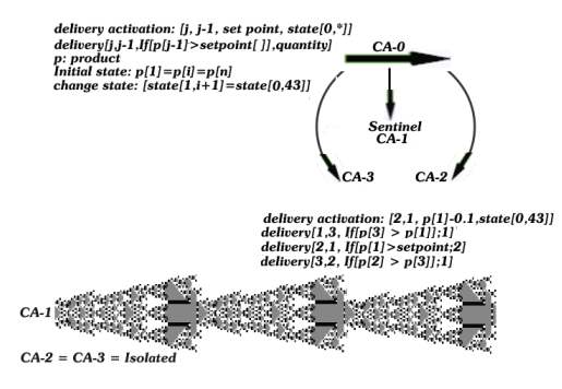
We continue with the directed loop. Three functions control CA behavior:

1. delivery activation[j,0, set point, state[0, i]]
2. delivery[j, j-1, If[pa[1] > setpoint; quantity]
3. change state[state[j, i+1]] = state[0,i]]

Initially CA do not exchange resources since the set point is high . When CA-0, reaches state i, it diminishes the set point and activates CA-1 delivery. In the present experiment delivery is initiated when CA-0 state= 43 (=[0, 43]). The amount of resources which CA-2 and CA-3 deliver is small and their structure does not change. When CA-0 reaches state=43, it initiates a change state, and CA-1 gets its final structure (solution).

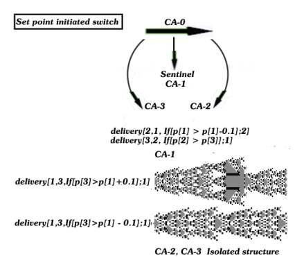
Set point initiated switch

In the next experiment the delivery conditions of CA-3 and CA-1 are the same. The quantity delivered by CA-3 = 1, and it does not change CA-3 structure. Only CA-2 structure fluctuates. However when CA-3 delivery condition is p[3] > p[1] - 0.1, CA-1 assumes the isolated structure. It is the sign of 0.1 which determines the CA-2 structure. When positive, CA-1 assumes its special structure, and when negative, (-k1) CA-1 displays the isolated structure.

This property is applied to create a flip-flop where CA-1 and CA-2 control each other.

The delivery condition of CA-2 may contain either -0.1 or +0.1. As the number switches between the positive and the negative, it determines CA-1 and CA-2 structure. The first intervals are somewhat shorter, however later on the CA assume their final solutions, which are complementary to each other.